
Estimating Uncertainty and Risk in Sales Forecasts and Budgets
Blaine Bateman
You can download a PDF version of this paper here.
The uncertainty and attendant risk in sales forecasts used in corporate budgeting processes is often ignored. The pervasive use of single-value forecasts (Savage, 2012) to “roll up” a forecast for the firm ignores important aspects of asymmetry that is likely present in each individual forecast provided by sales managers. The best way to estimate the rolled up forecast is by performing a Monte Carlo simulation, after representing the input forecasts as distributions. Fortunately, this can be relatively simple even using Microsoft Excel™ (Excel™) as the simulation tool. In this paper we motivate why this approach adds value and describe methods to implement the approach. We present some simple example cases to illustrate the difference between likely risks (both high and low) of missing the forecast and the risk that many managers may assume. Characterizing the actual risks based on a distribution can help firms better manage business risk and communicate with stakeholders.
Firms generally have an annual budgeting cycle, which begins with collecting forecasts for the next year from all the sales functions [1]. Whether a top-down [2] revenue target is given in advance or not, it is common, after finalizing all bottom-up sales inputs, to include additional revenues in the target for the next year--these additional revenues may be referred to as “stretch” or some other colorful adjective, with the meaning that the leadership expects sales to find additional revenue beyond that which can be forecast specifically.
It might be tempting to think of the stretch revenue as the uncertainty [3] in the forecast. While it is almost a given that the added top-down revenue is part of the total uncertainty in the forecast, in practice it is only a portion. In this paper I discuss uncertainty in the individual inputs, how to describe those inputs as distributions, the resulting total uncertainty by combining inputs with uncertainties and distributions, and finally how to model the distribution for the rolled-up forecast to estimate the total uncertainty.
Let’s first consider the case of a particular sales manager, we’ll call her Sharon, providing input into the forecast. For simplicity, we take the case where the initial input contains no “stretch”; i.e. it is the sum of specifically forecasted amounts by Sharon. Although there are invariably large data sets underlying the forecasts provided by sales managers, and the content of those detailed data may be adjusted many times during the process, in the end there is a single figure, FSharon, that represents Sharon’s contribution to the overall forecast. In most budgeting processes, that is as far as it goes, aside from later adjustments as already noted. Now, what if we asked Sharon if she was 100% confident in the figure FSharon? Generally, the answer would be “no”. A problem arises if we ask Sharon “how confident are you in your forecast?”. The question and hence the answer are ambiguous and can be interpreted in various ways. For instance, if Sharon responds “I am 75% confident”, she might be saying there is only 25% chance the real revenues will come in below FSharon. Alternatively, she might be saying that if you constructed a normal distribution representing the actual sales, with mean FSharon, then the ± 3 s limits would be ± 37.5% of the mean, or s = 12.5%. While the second response seems somewhat illogical, nonetheless there is a better way, and perhaps more commonly used way, to ask about the uncertainty of the forecast.
A better question for Sharon would be “what are your 90% confidence interval limits on FSharon, and what is the most likely value of the actual sales?” The answer to this question must be a range, and we note that the most likely (or expected) value can lie anywhere within this range. This leads us to another problem: most managers, if they envision a distribution of actual outcomes related to FSharon at all, they would almost always assume a symmetric, normally shaped (i.e. Bell Curve shaped) distribution with mean at FSharon. If we consider answers to the confidence interval question, Sharon might respond “the lower value is FℓSharon, the upper value is FuSharon, and the most likely value is F’Sharon.” We note that F’Sharon may not be equal to the FSharon given earlier. Why might that be the case?
Perhaps Sharon has a key account, and that account represents a large fraction of her total forecast. Sharon knows the customer has some expansion plans hinging on a few key deals. If they all are closed, then the total forecast might increase 25%. Sharon thinks less than half of these are very likely, but if they all are closed, then FuSharon moves up but the most likely value and the lower bound are unchanged. In fact, it is likely that most sales forecasts have asymmetric distributions of the possible actual values. Another case, for instance, might be a few large pending sales representing a significant downside. Yet another variant might consider capacity constraints that would require capital approval should the sales deals close, and the timing of capital expense (capex) approval and deployment affecting the current year forecast. To simplify thinking about this, just ask yourself “how many times has the upside been identical to the downside?”
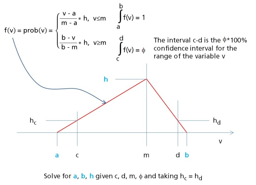
Now if we do ask Sharon for her forecast as a 90% confidence interval and a most likely value, what are we to do with those figures? It is common to use a triangular distribution to represent the distribution of possible outcomes like the sales forecast scenarios described above (Kacker, 2007) (Larham, 2010) (Palomo & Insua, 2004) (Rodger, 1999). In all references I reviewed discussing triangular distributions, I found the distribution is characterized by three values—the worst case, the best case, and the expected value. Consider what these values represent in terms of uncertainty: the lower and upper values imply the forecaster is 100% certain no values will occur either below the worst case or above the best case; in other words the sales manager gives you a range with no uncertainty about it. As already explained, a more likely case is that the sales manager can estimate a range representing a confidence interval of the actual values, say 90%, and a most likely or expected value. This case is illustrated in Figure 1.
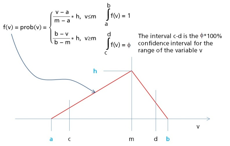
Figure 1. Probability distribution representing the distribution of possible actual sales based on the estimates of the sales manager. The values c, d, and m are given by the manager, as well as the confidence level. The values a, b, and h must be determined to characterize the distribution for use in risk estimation later.
Continuing with our sales manager Sharon, figure 1 says she is 90% confident the actual sales will fall between the value c and d, and thinks the most likely outcome is m. Mathematically, the area under the curve between c and d equals 0.9 or 90%. We also note that the area under the entire curve from a to b equals 1 or 100%. For a complete description of the probability distribution of actual sales outcomes, we need to find the values a, b and m, where m is the maximum height, which by definition must occur at the most likely outcome, m.
There are various ways we can approach the solution to the math/geometry problem of figure 1. In appendices A through C we outline some solutions approaches and develop two different solutions. For our purposes here, we note that we make use of the assumption that the height of f(v) is the same at c as it is at d (this is referred to in Appendix A as the “equal heights” assumption). In short, with the equal heights assumption we can find the unknown values easily using Excel™. With that in hand, let’s explore the implications of using triangular distributions in a rolled up forecast instead of point values.
We start with five forecasts submitted to be rolled up into a higher level forecast. These might represent five sales managers’ input into a business unit forecast, or five business units input into a company forecast. Table 1 shows the starting values.
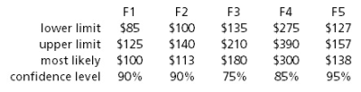
Table 1. Five sample forecasts to be used in the rolled-up forecast. The values are interpreted as follows. For F1, the forecaster is 90% confident that the actual sales will fall between $85M and $125M, and believes the most likely actual sales will be $100M.
These data are based on the premise that forecasts do have a range of possible values, and the managers providing the forecasts can provide at least some estimate of a confidence interval. Using the data in Table 1, we first solve for the unknown limit values, assuming the probability distributions of the input forecasts are represented by triangular distributions, as explained earlier.
Table 2. Solutions for the triangular distributions for five different input forecasts.
Interpretation of the results in Table 2 using the F3 data is that the input was a range of $135M to $210M at 75% confidence level, with a most likely value of $180M. Solving for the triangular distribution for F3 gives the worst case of $90M and best case of $240M. We can now use the defined triangular distributions together in a Monte Carlo simulation to estimate the probability distribution of the rolled-up forecast.
When the intervals are not symmetric the results can diverge from intuition quite dramatically. In addition, if the five inputs are independent of one another, the resulting probability distribution can be significantly different than many managers’ expectations. Figure 2 shows the results of a Monte Carlo simulation of the five test cases, where the distribution was generated from 40,000 [4] trials run in Microsoft Excel™ 2010.
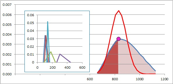
Figure 2. Monte Carlo Simulation results using the five test cases. The test distributions are shown in the inset. The red curve represents the implicit assumption about the outcome by management (see text). The blue curve is the distribution from the Monte Carlo simulation; the dark shaded area is the area to the left of the most likely value. Results generated using the equal heights assumption.
 The striking features of figure 2 are that while the most likely value of the simulated distribution is close to the sum of the five input values [5], the distribution differs from a normal distribution, and the distribution has a wider range of outcomes than many managers would expect. The likelihood of coming in below budget is about 40%, considerably more than the 15% that might be assumed in our example. On the other hand, the upper limit to the possible values is much higher than might otherwise be assumed, and there is more chance of upside than downside.
By examining the shapes of the input distributions and performing comparisons over time to actual results, it is possible to draw some conclusions about the quality of the individual forecasts. A common issue in sales forecasting are managers who desire to avoid “missing their number”. This leads to the phenomenon known as “sandbagging”, wherein the sales managers deliberately understate the most likely value. On the other hand, they may be similarly tempted to provide an excessively wide range of values as their confidence interval. If you ask a sales manager for a range of actual sales they have 90% confidence in, and you then ask them “what is the chance sales will come in below your low figure”, and their answer is “there is no chance my sales will be below the low figure”, then they are not providing an accurate range. Over time, enough empirical evidence may be accumulated to allow adjustments to input forecasts based on past forecasts vs. actual sales.
From a risk perspective, the example given here indicates a larger upside and the resulting distribution is skewed above the most likely value. An interesting situation to consider is if the values towards the higher end of the distribution might represent more sales than available capacity to deliver product, thus exposing the business to another risk. Perhaps capitalizing on the upside requires new capital to be obtained and installed, and there is a lead time for both review and approval, and purchase, delivery, and installation. The firm, looking at such a distribution, may choose to initiate a capital approval process earlier than normal to avoid missing out on upside sales.
Further, it should be stressed that in this example, there is a 40% chance of the actual sales coming in at some figure below the most likely value. Since the most likely value is probably used as the sales target, and may be communicated to other stakeholders, it would be sensible to state the target as a range with some confidence and a most likely value, or at least to state the chance of missing the value low.
In conclusion, we have illustrated why forecast inputs are better represented as distributions than point values. We have developed the process to easily represent these inputs as triangular distributions, making them available to a Monte Carlo simulation of the total forecast. Using the Monte Carlo approach, we have illustrated how to quantify risk of the actual sales coming in either below or above the forecast most likely value. This knowledge can be used to improve management processes in several ways, including a better understanding of downside risk and how that should be communicated to stakeholders.
Bibliography
Kacker, R. N. (2007). Trapezoidal and traingular ditributions for Type B evaluation of standard uncertainty. Metrologia 44, 117-127.
Larham, R. (2010, 11 27). Project Costing with the Triangular Distribution and Moment Matching. Retrieved 04 05, 2013, from Academia.edu: http://www.academia.edu/362251/Project_Costing_with_the_Triangular_Distribution_and_Moment_Matching
Palomo, J., & Insua, D. R. (2004, 02 24). Dynamic Models with Expert Input wtih Applications to Project Cost Forecasting. Retrieved 04 05, 2013, from Statistical and Applied Mathematical Sciences Institute: http://www.samsi.info/sites/default/files/tr2004-02.pdf
Rodger, C. a. (1999, 04 01). Uncertainty and Risk Analysis. Retrieved 04 05, 2013, from Metropolitan State University of Denver: http://clem.mscd.edu/~mayest/Excel/Files/Uncertainty%20and%20Risk%20Analysis.pdf
Savage, S. L. (2012). The Flaw of Averages: Why We Underestimate Risk in the Face of Uncertainty. Hoboken, New Jersey: John Wiley & Sons.
Appendix A. Alternative methods to find the endpoints and height of the triangular distribution representing a sales forecast.
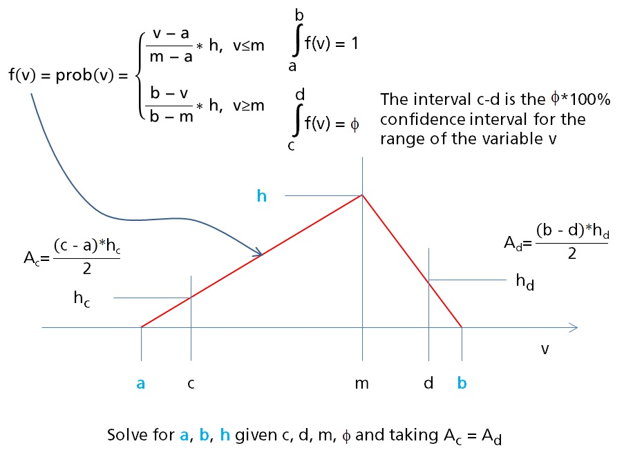
Figure A1. A triangular distribution where the values representing a confidence interval for v are given by c and d, along with the most likely (expected) value (m).
To solve this problem we can make use of the property of a triangular distribution:
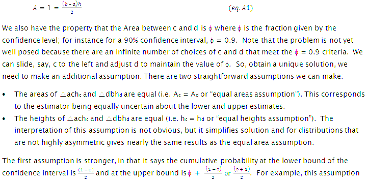 means that, for a 90% confidence interval, the cumulative probability at point c is 5% and at point d is 95%, which is intuitively correct. However, this approach is ill-defined if the distribution is a right triangle, because one of the small-triangle areas becomes zero. A possibility in the case of a right triangle is to assume the area of the corresponding small triangle is zero, then derive a solution. This may be reasonable if the actual circumstances warrant concluding that no values beyond the limit on the right angle side of the distribution are likely.
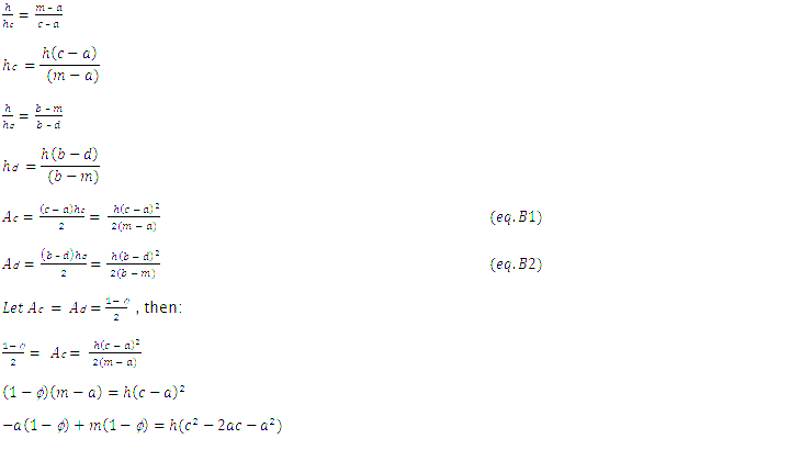
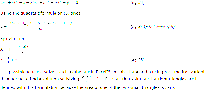
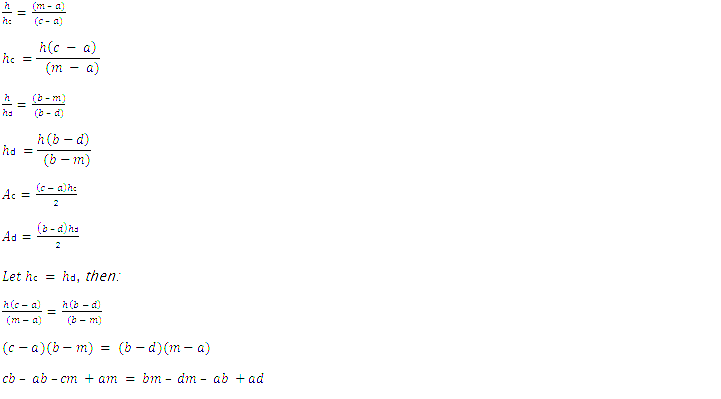
On the other hand, if we assume the values of the probability function are the same at the lower and upper ends of the confidence interval, that is, hc = hd, then we can generate expressions that are well behaved even for right triangles. Assuming hc = hd means that the probability is the same for v having the value c or having the value d. The interpretation of this constraint is not clear, because in many cases the cumulative probability at c and from d to b will not be equal. For practical purposes, this assumption may be good enough for the kinds of approximations needed for forecasting, as will be shown by examples below.
The solution using the first assumption (equal areas) proceeds as follows. Using the fact that the
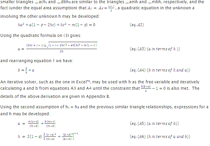
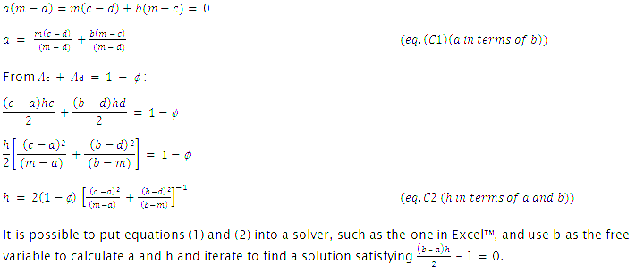
As before, this set of equations can be iteratively solved, using b as the free variable. The details of the second derivation are given in Appendix C.
To illustrate, we examine a case where the sales manager provides us with a 90% confidence interval of $105,000 to $160,000, and an expected value of $113,000. Using the equal heights assumption, the solver in Microsoft Excel™ 2010 gives a solution of a = $101,300; b = $181,736 and h = 0.025, as shown in Table A1.
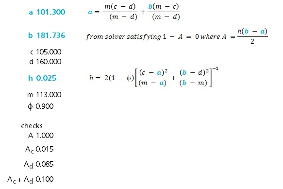
Table A1. Solution for the case where a 90% confidence interval is given as $105,000 to $170,000, the expected value is $113,000, and the equal heights assumption is used.
Note that the cumulative probability at the expected value is the chance of the actual value being below the expected value. This value can be calculated as the area of the left half of the distribution:
 Thus, in this example, there is about a 15% chance the actual sales come in below the expected value, or in other words it is much more likely the actual sales revenues come in high than low.
To use the resulting distributions in a simulation we would create the equations for the distribution:
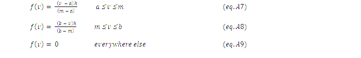
For each distribution in the simulation the corresponding values of a, b, and h are then substituted in equations (A7), (A8), and (A9).
Solving the same problem using the equal areas assumption generates the results shown in Table A2.
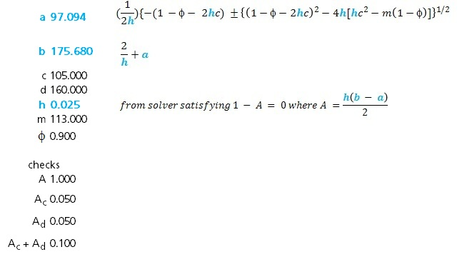 Table A2. Solution for the case where a 90% confidence interval is given as $105,000 to $170,000, the expected value is $113,000, and the equal areas assumption is used.
In this solution, the height of the probability distribution at the expected value is 0.025, the same as the solution using the equal heights assumption. The probability of the actual sales coming in below the expected value is:
 or in this case we estimate about a 20% chance that the actual sales come in below the expected value.
This example shows a 5% deviation between the two assumptions in the predicted likelihood of sales coming in low, which may not be important considering the range of sales estimated at 90% confidence level was from 7% below the expected value to as much as 42% above the expected value. The estimated distribution for the equal areas case is shown in Figure A2.
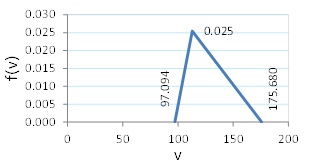
Figure A2. The resulting shape of the distribution for the two preceding examples is nearly a right triangle, which leads to significant deviations between the two methods.
Appendix B. Derivation of one solution using the assumed equal areas Ac = Ad.

By similar triangles:
Appendix C. Derivation of one solution using assumed equal heights hc = hd.
By similar triangles:
 Notes
Notes
[1] In this paper we consider any functions responsible for make sales to customers, and thereby generating revenue, to be sales functions, or simply sales. The budgeting cycle includes not only sales inputs but cost inputs as well; however in this paper we look only at the revenue side of the complete cycle. Also, while such processes are commonly iterative, for simplicity we assume there are a known set of sales inputs included in the final revenue total, and ignore the intervening changes to the individual forecast elements. While such iterations can introduce additional uncertainties into the forecasts, we further assume that each component in the final forecast can be described by a function that can comment on the uncertainty of the value included in the final forecast.
[2] When we refer to “rolled-up” forecast we mean simply the final total sales forecast figure from summing together all the individual submissions, after changes, plus any additions. When we refer to “bottom-up” forecasts we are referring simply to the individual submissions, after changes.
[3] As will become evident later, uncertainty refers to the concept that a single value for a forecast does not represent the full picture because there is a significant chance the actual revenues realized will differ from the forecast.
[4] In a Monte Carlo simulation, the input distributions are randomly sampled to obtain particular values of the actual sales for each trial, which are summed to obtain the total sales for that trial. This process is repeated thousands of times and the resulting values are plotted in a histogram to represent the estimated distribution of actual sales. In this case, a random number between 0 and 1 is generated and used as the cumulative probability for that trial; that is, the point along the distribution where the area under the curve equals the random value. Using the known distributions, the value of actual sales corresponding to the given cumulative probability can be determined for each distribution. These values are then summed.
[5] Note that regardless of the distribution shapes, we can add the most likely values of each distribution together and this sum is the most likely value of the distribution of all sales. In practice, in a Monte Carlo simulation the simulated value and the actual value might deviate slightly due to imperfect randomness of the sampling, or poor choice of the “bin” values of the resulting histogram. In the example in this paper, we constructed the histogram bins to be symmetric about the most likely value, to avoid an artifact created by forcing the largest bin to be below or above the most likely value.